Derivation of Hofstadter’s butterfly
Published:
We consider tight-binding model applied on a square lattice with lattice constant \(a\) whose sites are located at \((x, y) = (ma, na)\). We assume \(0 \le m, n < L\) so the system size is \(N = L^2\). The system is subjected to an external magnetic field along \(z\) direction, and here we choose the Landau gauge \(\vec{A} = (0, B x, 0)\). In the presence of magnetic field, the hopping terms transform as
\[\begin{aligned} - t e^{-i \frac{e}{\hbar c} \vec{A} \cdot (\vec{r}_1 - \vec{r}_2)} &= - t e^{-i \frac{2 \pi}{\phi_0} B x \vec{e}_y\cdot (\vec{r}_1 - \vec{r}_2)} \\ &= \begin{cases} - t & \text{hopping in } x \text{ direction} \\ - t e^{i 2 \pi \frac{B a^2}{\phi_0} m} = t e^{i 2 \pi \frac{\phi}{\phi_0} m} = t e^{i 2 \pi \alpha m} & \text{hopping in } y \text{ direction} \end{cases} \end{aligned}\]We hence obtain the Hamiltonian for system as follows
\[H = \sum_{m, n} \left( - t a^\dagger_{m + 1, n} a_{m, n} - t e^{i 2 \pi \alpha m} a^\dagger_{m, n + 1} a_{m, n} \right) + \text{h.c}.\]We will perform the Fourier transformation to the field operators \(a^\dagger\) and \(a\)
\[a_{m, n} = \frac{1}{N} \sum_{k_x, k_y} e^{i k_x m a + i k_y n a} b_{k_x, k_y},\]where \(-\frac{\pi}{a} \le k_x, k_y < \frac{\pi }{a}\).
Because of the Landau gauge, the hopping term in the \(x\)-direction is not affected by the magnetic field. Its Fourier transformation is therefore straightforward as
\[- t \sum_{m, n} a^\dagger_{m + 1, n} a_{m, n} + \text{h.c}= \sum_{m, n} -2 t \cos(k_x a) b^\dagger_{k_x, k_y} b_{k_x, k_y}\]On the other hand, the hopping term in \(y\) direction is affected by the magnetic field, it transforms as follow
\[\begin{aligned} \sum_{m, n} - t e^{i 2 \pi \alpha m} a^\dagger_{m, n + 1} a_{m, n} + \text{h.c} &= \frac{- t e^{i 2 \pi \alpha m}}{N^2} \sum_{k_x, k_y, k^\prime_x, k^\prime_y} e^{- i k_x m a - i k_y (n+1) a} b^\dagger_{k_x, k_y} e^{i k^\prime_x m a + i k^\prime_y n a} b_{k^\prime_x, k^\prime_y} + \text{h.c}\\ &= \frac{-t}{N^2}\sum_{k_x, k_y, k^\prime_x, k^\prime_y} e^{i \left(k^\prime_x - k_x + \frac{2 \pi \alpha m}{a}\right) m a} e^{ i \left(k^\prime_y - k_y\right)na}e^{- i k_y a} b^\dagger_{k_x, k_y} b_{k^\prime_x, k^\prime_y} + \text{h.c}\\ &= \sum_{k_x, k_y} -t e^{-i k_y a} b^\dagger_{k_x - \frac{2 \pi \alpha}{a}, k_y} b_{k_x, k_y} - t e^{i k_y a} b^\dagger_{k_x + \frac{2 \pi \alpha}{a}, k_y} b_{k_x, k_y}. \end{aligned}\]The total Hamiltonian now takes the following form
\[H = \sum_{k_x, k_y} -2 t \cos(k_x a) b^\dagger_{k_x, k_y} b_{k_x, k_y} -t e^{-i k_y a} b^\dagger_{k_x - \frac{2 \pi \alpha}{a}, k_y} b_{k_x, k_y} - t e^{i k_y a} b^\dagger_{k_x + \frac{2 \pi \alpha}{a}, k_y} b_{k_x, k_y}.\]We notice that \(k_x\) is being shifted by an amount of \(\frac{2 \pi \alpha}{a}\). Let us apply the following variable change, \(\) with $0 \le m < L$, as a result the first BZ along \(k_x\) is changed as \(- \frac{\pi}{a L} \le k_x < \frac{\pi}{a L}\). One should notice that with such variable change, if the ratio of unit-cell flux is a rational number, i.e \(\alpha = p/q\), \(k_x\) is periodic with period \(q\). The Hamiltonian is rewritten as
\[\begin{aligned} H = \sum_{k_x, k_y} &-2 t \cos\!\left(k_x a + \frac{2 \pi \alpha m}{a}\right) b^\dagger_{ k_x + \frac{2 \pi \alpha m}{a}, k_y} b_{ k_x + \frac{2 \pi \alpha m}{a}, k_y} \\ &-t e^{-i k_y a} b^\dagger_{ k_x + \frac{2 \pi \alpha (m-1)}{a}, k_y} b_{ k_x + \frac{2 \pi \alpha m}{a}, k_y} - t e^{i k_y a} b^\dagger_{ k_x + \frac{2 \pi \alpha (m+1)}{a}, k_y} b_{ k_x + \frac{2 \pi \alpha m}{a}, k_y}. \end{aligned}\]Assume the eigenstates can be written in the form of
\[\left| \psi \right\rangle_{k_x, k_y} = \sum_{m = 0}^{L -1} A_m \, b^\dagger_{k_x + \frac{2 \pi \alpha m}{a}, k_y} \left| 0 \right\rangle,\]one can derive a system of \(L\) equations, in which the \(m^{\text{th}}\) equation is written as
\[-2 \cos(k_x + 2\pi \alpha m) A_m - e^{-i k_y} A_{m - 1} - e^{i k_y} A_{m+1} = \epsilon A_m,\]here \(\epsilon = E/t\) and \(a = 1\) for simplicity. Before constructing the matrix for general \(q\), we first examine several small-\(q\) cases which can be solved analytically. In the case \(q = 1\) (or \(R\alpha = \phi/\phi_0 = 1\) equivalently), according to the periodic condition we have \(A_0 = A_{0+1} = A_{0-1}\), the solution of energy is straightforwardly computed as
\[\epsilon = - 2 \cos k_x - e^{-i k_y} - e^{i k_y} = -2 \cos k_x -2 \cos k_y.\]In the case \(q = 2\) (or \(\alpha = \phi/\phi_0 = 1/2\)), there are 2 energy bands corresponding to the eigenvalues of the following \(2\times 2\) matrix
\[\begin{pmatrix} -2 \cos(2 \pi \alpha \cdot 0 + k_x) & - e^{-i k_y} - e^{i k_y} \\ - e^{-i k_y} - e^{i k_y} & -2 \cos(2 \pi \alpha \cdot 1 + k_x) \end{pmatrix} \quad\Rightarrow\quad \epsilon = \pm 2 \sqrt{\cos^2 k_x + \cos^2 k_y}.\]In the case of general \(q\), there exists exactly \(q\) energy bands as they are the eigenvalues of a \(q \times q\) matrix
\[\begin{pmatrix} -2 \cos (2 \pi \alpha \cdot 0 + k_x) & - e^{i k_y} & 0 & \cdots & e^{-i k_y} \\ - e^{-i k_y} & -2 \cos (2 \pi \alpha \cdot 1 + k_x) & - e^{i k_y} & \cdots & 0 \\ 0 & - e^{-i k_y} & -2 \cos (2 \pi \alpha \cdot 2 + k_x) & \cdots & 0 \\ \vdots & & & \ddots & \vdots \\ e^{i k_y} & & & \cdots & -2 \cos (2 \pi \alpha \cdot (q- 1) + k_x) \end{pmatrix}.\]Notice that the periodic boundary condition is encoded by the position of \(e^{i k_y}\) at the bottom left of the matrix and its conjugated element.
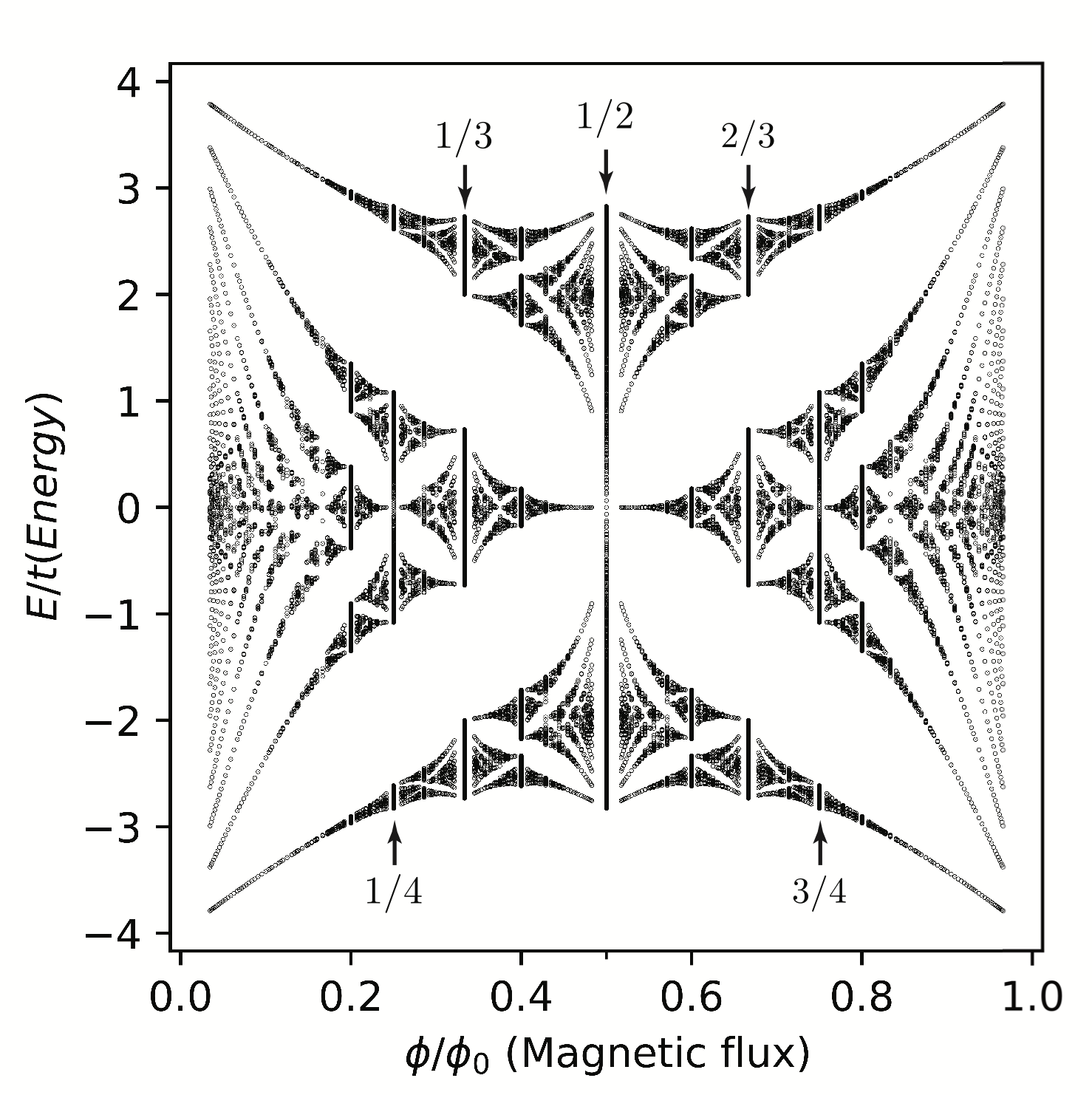
I numerically solved the above matrix for various data points of \(k_x\) and \(k_y\) to obtain such Hofstadter’s butterfly.